This article aims to analyze simulated degradation data using the r2IGP package. It covers the simulation of degradation paths, statistical inference through the EM algorithm and MLE, and visualization of model behaviors. The goal is to provide insights into parameter estimation and model evaluation for degradation modeling in reliability analysis.
# Load necessary packages for simulation and analysis
library(r2IGP)        # Main package for the analysis
library(magrittr)     # Pipe operator for cleaner code
library(tidyverse)    # Collection of packages for data manipulation
library(ggplot2)      # Visualization library for plots
library(viridis)      # Color scales for ggplot2
library(cowplot)      # Additional plotting functions
library(ggsci)        # Scientific color palettes
library(statmod)      # Statistical modeling
library(plotly)
library(kableExtra)
Parameter Setting
# Define simulation parameters
n <- 10       # Number of products
m <- 40       # Number of observation times
types <- "pp" # Type of degradation model (pp: power x power)
alpha <- c(1.2, 0.8)
beta <- c(4, 1)
kappa <- 5
sigma2 <- 0.1        # Variance for noise

# Define time scale
t <- 0:m
# Define degradation path for each product (same time scale for all products)
t_list <- rep(list(t), n)
r <- c(0, rrIG(length(t) - 1, 10, 1))
u <- cumsum(r * diff(t)[1]) # usage scale
u_list <- rep(list(u), n)  # List for each product's usage scale

# Define random effects for each product
gamma <- rnorm(n, kappa, sqrt(sigma2))

# All parameters
para <- c(alpha[1], beta[1], alpha[2], beta[2], kappa, sigma2)
Simulate Data
The function sim.dat.path() simulates degradation data
using different models. The available models are: "M0",
"M1", "M2", "M3",
"M4". The model structures are detailed in our related
publications.
# Simulate data for model "M0"
sim_dat <- sim.dat.path(
   model = "M0",
   type = types,
   m = m,
   n = n,
   t = t_list,
   u = u_list,
   par = para,
   gamma = gamma
)
The degradation paths can be visualized. The left plot shows the effects of two scales on product degradation, while the right plot shows the final observed degradation data.
# Visualize degradation paths
path_re <- degradation.path.plot.summary(
  model = "M0",
  data = list(sim_dat$Y_t, sim_dat$X_t, sim_dat$Z_t),
  t = t, u = u
)
# Display the plots
cowplot::plot_grid(plotlist = path_re)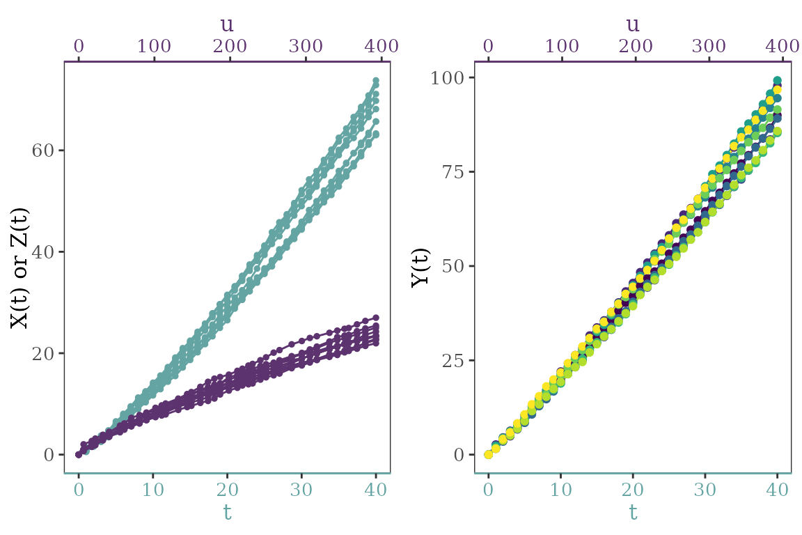
Degradation path.
# path.3D.plot(model="M0", units = 10, time = t, cycles = u, loss = sim_dat$Y_t) Statistical Inference
Initial Values
We use the Gauss-Legendre Quadrature method
(gaussian_legendre_integral()) for approximating the E-step
integration. Other methods like Trapezoidal Approximation
(trapezoidal_integral()) and Monte Carlo
Integration (mc_integral()) are also available.
# Define initial parameter values for different models
init_params_seq <- list(
  "M0" = rep(1, 6), "M1" = rep(1, 5),
  "M2" = rep(1, 6), "M3" = rep(1, 4),
  "M4" = rep(1, 3)
)

# Set model sequence
model_seq <- c("M0", "M1", "M2", "M3", "M4")

# Parameter settings
max_iter <- 5      # Maximum number of EM iterations
tol1 <- 10^-4       # Tolerance level
gl_point <- 30      # Number of points for Gauss-Legendre method
approx.method <- "gl" # Use Gauss-Legendre Quadrature method

# Initial parameter setup for each model
u_seq <- list(u_list, u_list, u_list, NULL, NULL, NULL, NULL) # M0,M1,M2,M3t,M3u,M4t,M4u
t_seq <- list(t_list, t_list, t_list, t_list, u_list, t_list, u_list)
We initialize parameters for different models based on their parameter structures and perform the EM algorithm.
EM Computation
This section performs parameter estimation for different models using
the Expectation-Maximization (EM) algorithm. For each model, initial
parameter values are generated via the init.guess()
function. The EM algorithm is then applied using the EM()
function, with the Gauss-Legendre Quadrature method
(gaussian_legendre_integral()) for E-step integration. For
models M6 and M7, the optim()
function is used for maximum likelihood estimation. The results are
stored in em_para_re, and if any errors occur during the
estimation, they are handled with tryCatch(), ensuring that
the process continues even if some models fail to converge.
data_store <- data_detail <- em_para <- em_iter_list <- inti_par <- list()
em_para_re <- vector("list", length(model_seq))

for (q in 1:length(model_seq)) {
  inti_par[[q]] <- init.guess(
    model = model_seq[q], types, data = sim_dat$diff_Y,
    t_list = t_seq[[q]], u_list = u_seq[[q]],
    init_param = init_params_seq[[q]]
  )
  if (q %in% c(6, 7)) {
    em_para_re[[q]] <- tryCatch(
      optim(inti_par[[q]], M4.loglik,
        types = types, t_list = t_seq[[q]],
        data = sim_dat$diff_Y
      )$par,
      error = function(e) rep(NA, 3)
    )
  } else {
    em_para[[q]] <- tryCatch(
      EM(
        data = sim_dat$diff_Y, par0 = inti_par[[q]], types = types,
        tol1 = tol1, max_iter = max_iter,
        t_list = t_seq[[q]], u_list = u_seq[[q]], model = model_seq[q], n_points = gl_point,
        approx.method = approx.method
      ),
      error = function(e) NA
    )
    em_para_re[[q]] <- if (any(is.na(em_para[[q]]))) rep(NA, length(init_params_seq[[q]])) else as.numeric(em_para[[q]]$par_re[em_para[[q]]$iter, ])
  }
}Note: Since a large number of iterations of the EM algorithm requires a certain amount of time, 50 is used as an example here (it has not actually converged yet). Readers are welcome to modify it according to their needs.
Log-Likelihood and AIC Calculation
Log-likelihood and AIC are calculated for model comparison.
loglik <- as.numeric()
for (q in 1:length(model_seq)) {
  loglik[q] <- round(
    Log.liklihod(
      model = model_seq[q],
      est_par = em_para_re[[q]],
      data = sim_dat$diff_Y,
      t_list = t_seq[[q]],
      u_list = u_seq[[q]],
      types = types
      ),
    3)
}
# AIC computation
aic <- 2 * length(sapply(em_para_re, length)) - 2 * loglik
which.min(aic)
#> [1] 1
Final Results
The final estimated parameters, log-likelihood, and AIC values are presented in a summarized table.
# Store and display final results
sim_para <- data.frame(
  "M0" = append(em_para_re[[1]], NA, after = 4),
  "M1" = append(em_para_re[[2]], rep(NA, 2), after = 5),
  "M2" = append(em_para_re[[3]], NA, after = 4),
  "M3t" = append(em_para_re[[5]], rep(NA, 3), after = 2),
  "M3u" = c(rep(NA, 2), append(em_para_re[[4]], rep(NA, 1), after = 2)),
  "M4t" = c(append(em_para_re[[6]], rep(NA, 2), after = 2), rep(NA, 2)),
  "M4u" = c(rep(NA, 2), em_para_re[[7]], rep(NA, 2))
)
final_sim_para <- data.frame(t(rbind(sim_para, loglik, aic)))
final_sim_para[7] <- sqrt(final_sim_para[7])
colnames(final_sim_para) <- c("alpha_t", "beta_t", "alpha_u",
                              "beta_u", "gamma", "kappa",
                              "sigma", "Loglik", "AIC")

# Display the table
kableExtra::kable(round(final_sim_para, 3))| alpha_t | beta_t | alpha_u | beta_u | gamma | kappa | sigma | Loglik | AIC | |
|---|---|---|---|---|---|---|---|---|---|
| M0 | 1.224 | 4.256 | 0.730 | 1.557 | NA | 5.601 | 0.286 | -112.512 | 239.024 |
| M1 | 1.215 | 4.232 | 0.724 | 1.543 | 5.352 | NA | NA | -117.382 | 248.764 |
| M2 | 1.222 | 4.253 | 0.728 | 1.555 | NA | 5.384 | 0.061 | -120.056 | 254.112 |
| M3t | 0.990 | 0.618 | NA | NA | NA | 2.507 | 0.108 | -168.955 | 351.910 |
| M3u | NA | NA | 1.092 | 7.215 | NA | 4.440 | 0.219 | -387.862 | 789.724 |
| M4t | 1.091 | 6.590 | NA | NA | 4.029 | NA | NA | -167.362 | 348.724 |
| M4u | NA | NA | 0.994 | 0.587 | 2.431 | NA | NA | -387.813 | 789.626 |